The Q: March Madness Seedigami

Quang Nguyen

March Madness is currently happening. Last night, I stumbled upon this tweet:

Seedigami! NC State is the first 11 seed to beat a 4 seed in NCAA tournament history pic.twitter.com/FbKcQ7Qwdi
— SaintArkweather (@SwordfishCFH) March 31, 2024

In case you’re not familiar, Scorigami is a fun concept in sports which refers to a game/match that finishes in a score that has not happened before in the history of a sport league. This can be applied to any sport, but perhaps it is most popular in American football, and there’s even a Twitter account devoted to NFL Scorigami.

The tweet above is a nice little spin-off of Scorigami. It is Scorigami, but for March Madness seeding, hence the name “Seedigami”. The purpose is to illustrate whether one seed has recorded a victory against other seeds in the history of the tournament. Last night, it was the first instance ever where an 11 seed (NC State) won a game against a 4 seed (Duke).

As soon as I saw this tweet, I immediately thought about making a slightly different version of it. That is, a heatmap showing how often each seed has beaten every other seed throughout the history of March Madness.

Here, let’s only consider every year starting from 1985, since the tournament was expanded to 64 teams that year. I can easily get the data from the famous March Machine Learning Mania Kaggle competition, whose 10th edition is in progress.

What I’ll need are the following tables (more detailed descriptions can be found in the data link above):

MNCAATourneyCompactResults: for game results
MNCAATourneySeeds: for seeding info

Now, I’ll (briefly) walk through my entire process of creating the desired heat map, starting with data preparation. First, let’s import the data and get a glimpse of both tables.

Show code

library(tidyverse)
library(janitor)
results <- read_csv("MNCAATourneyCompactResults.csv") |> 
  clean_names()
seeds <- read_csv("MNCAATourneySeeds.csv") |> 
  clean_names()

Show code

results

# A tibble: 2,451 × 8
   season day_num w_team_id w_score l_team_id l_score w_loc num_ot
    <dbl>   <dbl>     <dbl>   <dbl>     <dbl>   <dbl> <chr>  <dbl>
 1   1985     136      1116      63      1234      54 N          0
 2   1985     136      1120      59      1345      58 N          0
 3   1985     136      1207      68      1250      43 N          0
 4   1985     136      1229      58      1425      55 N          0
 5   1985     136      1242      49      1325      38 N          0
 6   1985     136      1246      66      1449      58 N          0
 7   1985     136      1256      78      1338      54 N          0
 8   1985     136      1260      59      1233      58 N          0
 9   1985     136      1314      76      1292      57 N          0
10   1985     136      1323      79      1333      70 N          0
# ℹ 2,441 more rows

Show code

seeds

# A tibble: 2,558 × 3
   season seed  team_id
    <dbl> <chr>   <dbl>
 1   1985 W01      1207
 2   1985 W02      1210
 3   1985 W03      1228
 4   1985 W04      1260
 5   1985 W05      1374
 6   1985 W06      1208
 7   1985 W07      1393
 8   1985 W08      1396
 9   1985 W09      1439
10   1985 W10      1177
# ℹ 2,548 more rows

Each tournament consists of 63 games. Notice that the data also include games from the First Four.

Show code

results |> 
  count(season) |> 
  arrange(- n)

# A tibble: 38 × 2
   season     n
    <dbl> <int>
 1   2011    67
 2   2012    67
 3   2013    67
 4   2014    67
 5   2015    67
 6   2016    67
 7   2017    67
 8   2018    67
 9   2019    67
10   2022    67
# ℹ 28 more rows

And TIL that the First Four used to be the “Opening round” (2001-2010), before the name was switched to First Four in 2011 and remains the same until now. These facts can be used in the data preparation process to keep only the 64 teams in the first round of every tournament.

Show code

# main 64-team field
results_main <- results |> 
  group_by(season) |>
  mutate(game_num = row_number()) |> # define game number for each tournament
  ungroup() |>
  filter(!(season %in% 2001:2010 & game_num == 1)) |> 
  filter(!(season %in% 2011:2023 & game_num %in% 1:4))

results_main |> 
  count(season) |> 
  arrange(n)

# A tibble: 38 × 2
   season     n
    <dbl> <int>
 1   2021    62
 2   1985    63
 3   1986    63
 4   1987    63
 5   1988    63
 6   1989    63
 7   1990    63
 8   1991    63
 9   1992    63
10   1993    63
# ℹ 28 more rows

Notice in 2021 there were only 62 games played instead of 63. I went back and check and found that there was a no-contest game between VCU and Oregon in 2021 due to COVID, which explains why there was 1 less game. (Now I do remember this.)

What I want now is a table with the seeds for the winning and losing teams in the data. This can be done by pivoting the results table and then joining it with the seeding table. Note that the ongoing 2024 tournament game results are not provided in the data, so I self-collected the 2024 results (as of today, up to the Elite 8). (The 2024 data can probably be obtained via a freely-available data resource such as the hoopR, ncaahoopR, or cbbdata R packages, to name a few.)

Show code

results_seeds <- results_main |> 
  select(season, w_team_id, l_team_id) |> 
  mutate(matchup = str_c(w_team_id, l_team_id)) |> 
  pivot_longer(ends_with("team_id"),
               names_to = "outcome",
               values_to = "team_id") |>
  mutate(outcome = str_remove(outcome, "_team_id")) |> 
  left_join(seeds)

results_seeds_w_l <- results_seeds |> 
  mutate(seed = str_remove_all(seed, "[:alpha:]"),
         seed = as.numeric(seed)) |> 
  select(-team_id) |> 
  pivot_wider(names_from = outcome,
              values_from = seed) |> 
  select(-matchup)

results24 <- tibble(
  season = 2024,
  w_l = c("1_16", "9_8", "5_12", "13_4", "11_6", "3_14", "7_10", "2_15",
          "1_9", "5_13", "3_11", "2_7", "1_5", "3_2", "1_3",
          "1_16", "9_8", "12_5", "4_13", "6_11", "3_14", "7_10", "2_15",
          "1_9", "4_12", "6_3", "2_7", "4_1", "6_2", "4_6",
          "1_16", "9_8", "12_5", "4_13", "11_6", "14_3", "10_7", "2_15",
          "1_9", "4_12", "11_14", "2_10", "4_1", "11_2", "11_4",
          "1_16", "8_9", "5_12", "4_13", "11_6", "3_14", "7_10", "2_15",
          "1_8", "5_4", "3_11", "2_7", "1_5", "2_3", "1_2")
) |> 
  separate(w_l, into = c("w", "l"), sep = "_", convert = TRUE)


results_seeds_w_l <- results_seeds_w_l |> 
  bind_rows(results24)

Now I have information on the winning and losing seeds for each game from 1985 up to today (April Fools’ Day - but no fooling…).

Show code

results_seeds_w_l

# A tibble: 2,453 × 3
   season     w     l
    <dbl> <dbl> <dbl>
 1   1985     9     8
 2   1985    11     6
 3   1985     1    16
 4   1985     9     8
 5   1985     3    14
 6   1985    12     5
 7   1985     5    12
 8   1985     4    13
 9   1985     2    15
10   1985     7    10
# ℹ 2,443 more rows

How often has each of these combinations happened?

Show code

results_seeds_w_l |> 
  count(w, l)

# A tibble: 128 × 3
       w     l     n
   <dbl> <dbl> <int>
 1     1     1    21
 2     1     2    38
 3     1     3    23
 4     1     4    48
 5     1     5    43
 6     1     6     9
 7     1     7     6
 8     1     8    61
 9     1     9    74
10     1    10     6
# ℹ 118 more rows

To handle the combinations that have never occurred, I create a table for every possible winning-losing seed combination, and then join with the existing table and update as needed.

Show code

# initialize with all zero's
all_matchups <- crossing(w = 1:16, l = 1:16, n = 0)
# join and update
all_matchups <- all_matchups |> 
  rows_update(count(results_seeds_w_l, w, l), by = c("w", "l"))
all_matchups

# A tibble: 256 × 3
       w     l     n
   <int> <int> <dbl>
 1     1     1    21
 2     1     2    38
 3     1     3    23
 4     1     4    48
 5     1     5    43
 6     1     6     9
 7     1     7     6
 8     1     8    61
 9     1     9    74
10     1    10     6
# ℹ 246 more rows

Now we can finally make the heat map.

Show code

all_matchups |> 
  ggplot(aes(w, l)) +
  geom_tile(aes(fill = n), color = "lightgray") +
  geom_text(aes(label = n, family = "Chivo"), size = rel(3)) +
  scale_x_continuous(breaks = 1:16) +
  scale_y_continuous(breaks = 1:16) +
  scale_fill_gradient2(high = "purple") +
  annotate("rect", 
           xmin = c(11, 15, 15, 3:5, 15, 16) - 0.5,
           xmax = c(11, 15, 15, 3:5, 15, 16) + 0.5,
           ymin = c(4, 3, 7, 3:5, 2, 1) - 0.5,
           ymax = c(4, 3, 7, 3:5, 2, 1) + 0.5, 
           color = "black", fill = "transparent", linewidth = 1) +
  labs(x = "\nWinning Seed",
       y = "Losing Seed\n",
       title = "March Madness Seedigami",
       subtitle = "How often does a seed beat another?") +
  theme_minimal(base_family = "Chivo") +
  theme(panel.grid = element_blank(),
        legend.position = "none",
        plot.title = element_text(hjust = 0.5),
        plot.subtitle = element_text(hjust = 0.5))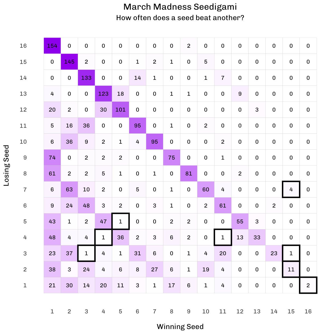

Some observations here:

The highlighted cells are those that I find interesting.
Teams don’t beat opposing teams with the same seed number that frequently (a 3, 4, and 5 have beaten their corresponding similarly-seeded opponent only once).
A 15 has beaten a 2 11 times. My favorite was Middle Tennessee beating Michigan State in 2016 (my first year following March Madness).
More interesting facts about the 15 seed: They’ve also beaten a 3 seed once (Saint Peter’s vs Purdue in 2022) and a 7 seed four times (which makes sense, given how often a 2 is beaten in the first round).
As previously mentioned, NC State vs. Duke (11 vs. 4) yesterday was the latest Seedigami.
And of course, the two famous 16 vs 1 upsets. (Will Purdue this year follow what Virginia did in 2019 - winning the title after being eliminated in the first round the year before?)

That’s it for now… Maybe more March Madness stuff to come… MAYBE.

How many days have passed since my last blog?

Show code

today() - as.Date("2022-12-19")

Time difference of 469 days

Until next time…

March Madness Seedigami

Citation