Over the past few weeks, I have been playing around with gganimate, a ggplot2 extension for making animated plots in R, and here is a collection of my recent data animations about the world of sports. The full code to each one of the graphs can be found below or on my GitHub. Feel free to suggest a new animation, or give me some feedback on my products. I’d highly appreciate them all.
Football: EURO 2020
The biggest sporting event in the world this summer prior to the Olympics is no doubt, the UEFA EURO 2020 (or to be more exact… EURO 2020ne). The following graphs contain information on past tournament performances of a storied national squad, and a roller-coaster EURO 2020 group stage.
England Performances
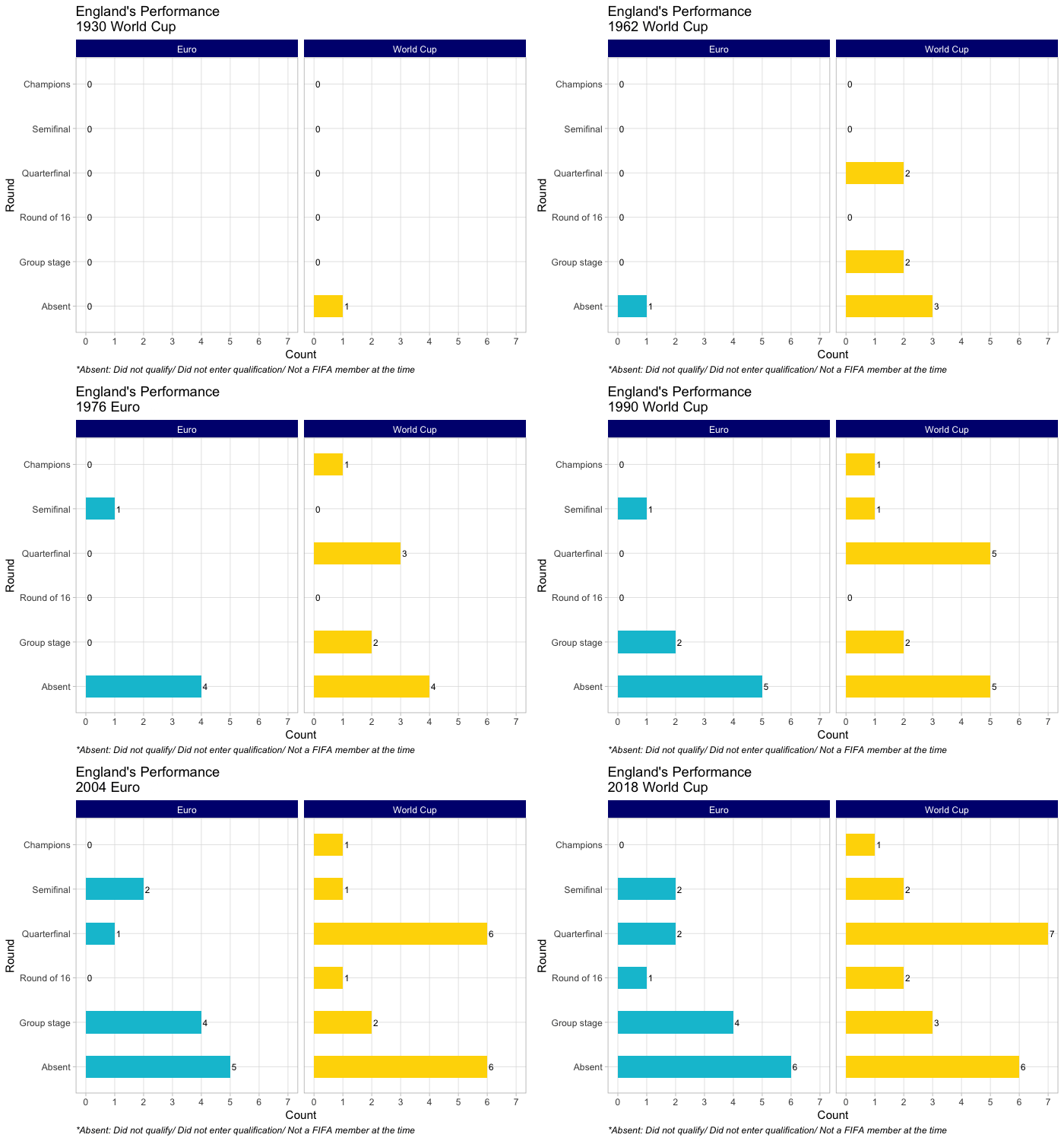
Will this finally be the year England fans have been waiting for for 55 years? Here is a view of England’s performance at major football tournaments (EURO and World Cup) prior to EURO 2020.
Show code
library(tidyverse)
library(gganimate)
library(rvest)
library(janitor)
theme_set(theme_light())

# scrape data from Wikipedia
eng_wiki <- "https://en.wikipedia.org/wiki/England_national_football_team"
eng_html <- read_html(eng_wiki)
eng_tables <- html_table(eng_html)

rounds <- c("Absent", "Group stage", "Round of 16", "Quarterfinal", "Semifinal", "Champions")
wc_years <- c("1930", "1934", "1938", seq(1950, 2018, 4))
euro_years <- as.character(seq(1960, 2016, 4))
years <- sort(c(wc_years, euro_years))

eng_wc <- eng_tables[[37]] %>%
  row_to_names(row_number = 1) %>%
  select(Year, Round) %>%
  filter(Year %in% wc_years) %>%
  mutate(Round = if_else(str_detect(Round, "(?i)not") == TRUE, "Absent", Round),
         Round = str_remove(Round, "-"),
         Round = str_replace(Round, "finals", "final"),
         Round = if_else(Round %in% c("Third place", "Fourth place"), "Semifinal",
                         if_else(Round == "Second group stage", "Quarterfinal", Round)),
         Round = factor(Round, levels = rounds)) %>%
  add_count(Year, Round, name = "Count") %>%
  mutate(Year = factor(Year, levels = years))

eng_wc <- full_join(eng_wc, expand(eng_wc, Year, Round)) %>%
  mutate(Count = ifelse(is.na(Count), 0, Count)) %>%
  arrange(Year, Round) %>%
  group_by(Round) %>%
  mutate(Count = cumsum(Count),
         Tournament = "World Cup")

eng_euro <- eng_tables[[39]]  %>%
  row_to_names(row_number = 1) %>%
  select(Year, Round) %>%
  filter(Year %in% euro_years) %>%
  mutate(Round = if_else(str_detect(Round, "(?i)not") == TRUE, "Absent", Round),
         Round = str_remove(Round, "-"),
         Round = str_replace(Round, "finals", "final"),
         Round = if_else(Round %in% c("Third place", "Fourth place"), "Semifinal",
                         if_else(Round == "Second group stage", "Quarterfinal", Round)),
         Round = factor(Round, levels = rounds)) %>%
  add_count(Year, Round, name = "Count") %>%
  mutate(Year = factor(Year, levels = years))

eng_euro <- full_join(eng_euro, expand(eng_euro, Year, Round)) %>%
  mutate(Count = ifelse(is.na(Count), 0, Count)) %>%
  arrange(Year, Round) %>%
  group_by(Round) %>%
  mutate(Count = cumsum(Count),
         Tournament = "Euro")

eng_results <- eng_wc %>%
  bind_rows(eng_euro) %>%
  arrange(Year) %>%
  mutate(Year = if_else(Year %in% wc_years,
                        paste(Year, "World Cup"),
                        paste(Year, "Euro")))

eng_anim <- eng_results %>%
  ggplot(aes(x = Count, y = Round, fill = Tournament)) +
  geom_col(width = 0.5, show.legend = FALSE) +
  geom_text(aes(label = as.character(Count)), size = 3, hjust = -0.3) +
  scale_x_continuous(breaks = 0:7) +
  facet_wrap(~ Tournament) +
  scale_fill_manual(values = c("#00c1d5", "gold")) +
  theme(strip.background = element_rect(fill = "#00007e"),
        panel.grid.minor.x = element_blank(),
        plot.caption=element_text(hjust = 0, face = "italic")) +
  transition_states(Year, wrap = FALSE) +
  labs(caption = "\n*Absent: Did not qualify/ Did not enter qualification/ Not a FIFA member at the time",
       title = "England's Performance \n {closest_state}")

animate(eng_anim, nframes = 432, fps = 24, height = 500, width = 700, res = 100, end_pause = 60)
Group F’s Chaotic Final Day
Once again, shoutout to @statsinthewild for the suggestion:
@qntkhvn I have a data view idea.
— Volume Tweeter (@StatsInTheWild) June 23, 2021
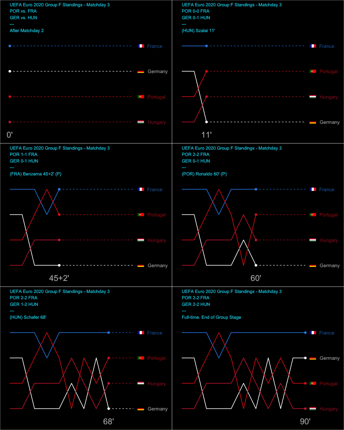
X axis is game time and y axis is the ranking of group F teams. Would be cool to see how it changed over the course of the games today.
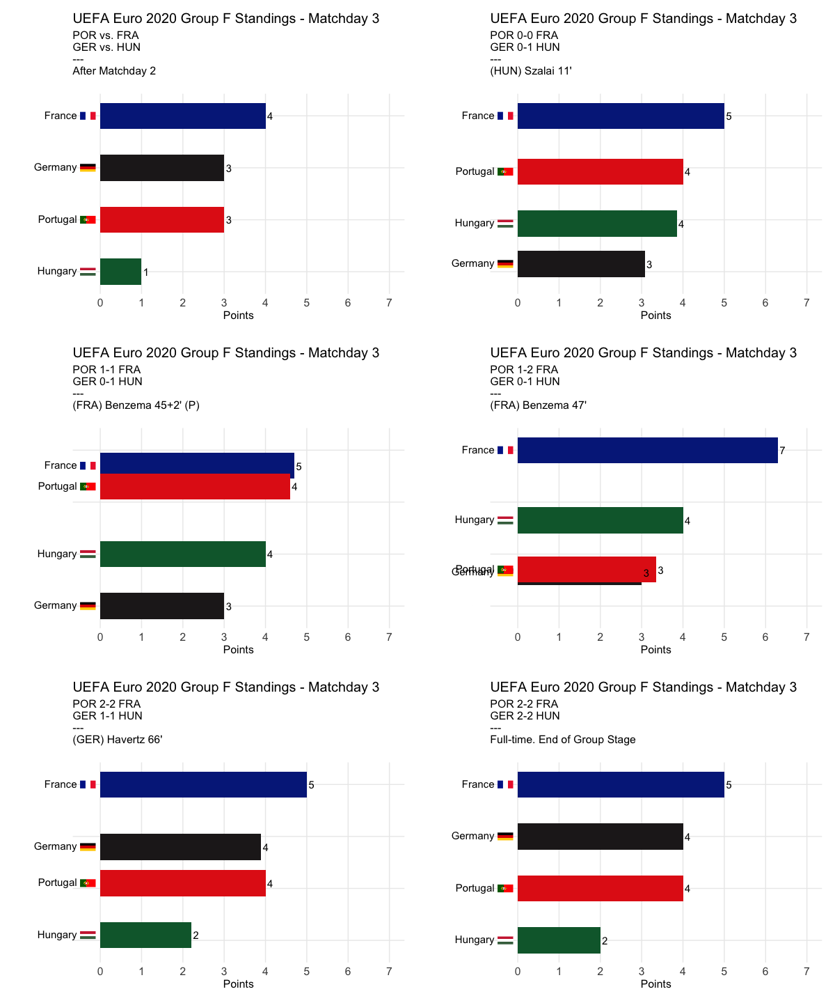
As referred to by many football experts and fans as the “group of death” of this year’s EURO, group F certainly lived up to the expectations. On the final day of the group stage where both group F matches started at the same time (here is the reason), every team was in a position to advance to the knockout stage at some point, and one team was in every position over the course of the matches! How wild!
Show code
library(countrycode)
library(ggflags)
library(ggdark)
theme_set(theme_minimal())

events <- c(
  "POR vs. FRA\nGER vs. HUN\n---\nAfter Matchday 2\n",
  "POR 0-0 FRA\nGER 0-0 HUN\n---\nKickoff\n",
  "POR 0-0 FRA\nGER 0-1 HUN\n---\n(HUN) Szalai 11'\n",
  "POR 1-0 FRA\nGER 0-1 HUN\n---\n(POR) Ronaldo 30' (P)\n",
  "POR 1-1 FRA\nGER 0-1 HUN\n---\n(FRA) Benzema 45+2' (P)\n",
  "POR 1-2 FRA\nGER 0-1 HUN\n---\n(FRA) Benzema 47'\n",
  "POR 2-2 FRA\nGER 0-1 HUN\n---\n(POR) Ronaldo 60' (P)\n",
  "POR 2-2 FRA\nGER 1-1 HUN\n---\n(GER) Havertz 66'\n",
  "POR 2-2 FRA\nGER 1-2 HUN\n---\n(HUN) Schafer 68'\n",
  "POR 2-2 FRA\nGER 2-2 HUN\n---\n(GER) Goretzka 84'\n",
  "POR 2-2 FRA\nGER 2-2 HUN\n---\nFull-time. End of Group Stage\n"
)

f <- tribble(
  ~Frame, ~Team, ~Points, ~Rank, ~GD,
  events[1], "France", 4, 1, 1,
  events[1], "Germany", 3, 2, 1,
  events[1], "Portugal", 3, 3, 1,
  events[1], "Hungary", 1, 4, -3,

  events[2], "France", 5, 1, 1,
  events[2], "Germany", 4, 2, 1,
  events[2], "Portugal", 4, 3, 1,
  events[2], "Hungary", 2, 4, -3,

  events[3], "France", 5, 1, 1,
  events[3], "Germany", 3, 4, 0,
  events[3], "Portugal", 4, 2, 1,
  events[3], "Hungary", 4, 3, -2,

  events[4], "France", 4, 2, 0,
  events[4], "Germany", 3, 4, 0,
  events[4], "Portugal", 6, 1, 2,
  events[4], "Hungary", 4, 3, -2,

  events[5], "France", 5, 1, 1,
  events[5], "Germany", 3, 4, 0,
  events[5], "Portugal", 4, 2, 1,
  events[5], "Hungary", 4, 3, -2,

  events[6], "France", 7, 1, 2,
  events[6], "Germany", 3, 3, 0,
  events[6], "Portugal", 3, 4, 0,
  events[6], "Hungary", 4, 2, -2,

  events[7], "France", 5, 1, 1,
  events[7], "Germany", 3, 4, 0,
  events[7], "Portugal", 4, 2, 1,
  events[7], "Hungary", 4, 3, -2,

  events[8], "France", 5, 1, 1,
  events[8], "Germany", 4, 2, 1,
  events[8], "Portugal", 4, 3, 1,
  events[8], "Hungary", 2, 4, -3,

  events[9], "France", 5, 1, 1,
  events[9], "Germany", 3, 4, 0,
  events[9], "Portugal", 4, 2, 1,
  events[9], "Hungary", 4, 3, -2,

  events[10], "France", 5, 1, 1,
  events[10], "Germany", 4, 2, 1,
  events[10], "Portugal", 4, 3, 1,
  events[10], "Hungary", 2, 4, -3,

  events[11], "France", 5, 1, 1,
  events[11], "Germany", 4, 2, 1,
  events[11], "Portugal", 4, 3, 1,
  events[11], "Hungary", 2, 4, -3
)

anim_bars <- f %>%
  mutate(Frame = factor(Frame, levels = events),
         Code = str_to_lower(countrycode(Team, "country.name", "iso2c"))) %>%
  ggplot() +
  geom_col(aes(x = Rank, y = Points, group = Team, fill = Team),
           show.legend = FALSE, width = 0.5) +
  geom_text(aes(x = Rank, y = 0, label = paste(Team, " ", " ", " ", " ", sep = " "),
                group = Team),
            hjust = 1, size = 4, vjust = 0.35) +
  geom_text(aes(x = Rank, y = Points, label = as.character(Points)),
            hjust = -0.3, size = 4) +
  geom_flag(aes(x = Rank, y = -0.3, country = Code), size = 6) +
  coord_flip(clip = "off") +
  scale_x_reverse() +
  scale_y_continuous(breaks = 0:9) +
  theme(
    axis.text = element_text(size = 12),
    axis.title = element_text(size = 12),
    axis.ticks = element_blank(),
    axis.title.y = element_blank(),
    axis.text.y = element_blank(),
    plot.margin = margin(0.5, 0.5, 0.5, 2.7, "cm"),
    panel.spacing.x = unit(5.5, "lines"),
    panel.grid.minor = element_blank(),
    strip.background = element_rect(fill = "#00c1d5", color = "#00c1d5"),
    plot.title = element_text(size = 15),
    plot.subtitle = element_text(size = 12)
  ) +
  scale_fill_manual(values = c("#052789", "#231f20", "#0b663a", "#e42518")) +
  transition_states(Frame, wrap = FALSE) +
  ease_aes("quadratic-in-out") +
  labs(
    title = "UEFA Euro 2020 Group F Standings - Matchday 3",
    subtitle = "{closest_state}"
  )

animate(anim_bars, nframes = 500, fps = 50, height = 480, width = 600, res = 95, duration = 15, end_pause = 100)
Show code
anim_lines <- f %>%
  mutate(
    Min = case_when(
      Frame == events[1] ~ "0'",
      Frame == events[2] ~ "1'",
      Frame == events[3] ~ "11'",
      Frame == events[4] ~ "30'",
      Frame == events[5] ~ "45+2'",
      Frame == events[6] ~ "47'",
      Frame == events[7] ~ "60'",
      Frame == events[8] ~ "66'",
      Frame == events[9] ~ "68'",
      Frame == events[10] ~ "84'",
      Frame == events[11] ~ "90'",
      TRUE ~ as.character(Frame)
    ),
    Code = str_to_lower(countrycode(Team, "country.name", "iso2c"))
  ) %>%
  ggplot(aes(x = Min, y = Rank, group = Team, color = Team)) +
  geom_line(size = 1) +
  geom_point(size = 3.5) +
  geom_text(aes(x = 12, label = Team), hjust = -0.1, alpha = 0.7, size = 6) +
  geom_text(aes(x = Min, y = 4.5, label = Min), alpha = 0.5,  col = "gray", size = 10) +
  geom_text(aes(x = 1, y = 0, label = paste0("UEFA Euro 2020 Group F Standings - Matchday 3\n", Frame)),
            hjust = 0, col = "#00c1d5", size = 5.5) +
  geom_segment(aes(xend = max(Min), yend = Rank), linetype = 2, size = 0.7) +
  geom_flag(aes(x = 11.6, y = Rank, country = Code), size = 8) +
  dark_theme_minimal() +
  theme(
    legend.position = "none",
    axis.title = element_blank(),
    axis.text = element_blank(),
    panel.grid.major = element_blank(),
    panel.grid.minor = element_blank(),
  ) +
  scale_y_reverse() +
  scale_color_manual(values = c("#318ce7", "white", "#CD2A3E", "#e42518")) +
  expand_limits(x = c(1, 14), y = -0.5) +
  transition_reveal(as.numeric(as.factor(Min))) +
  enter_fade() +
  exit_fade() +
  ease_aes('cubic-in-out')

animate(anim_lines, nframes = 500, height = 500, width = 600, fps = 50, end_pause = 100, rewind = FALSE)
Daily Group Tables
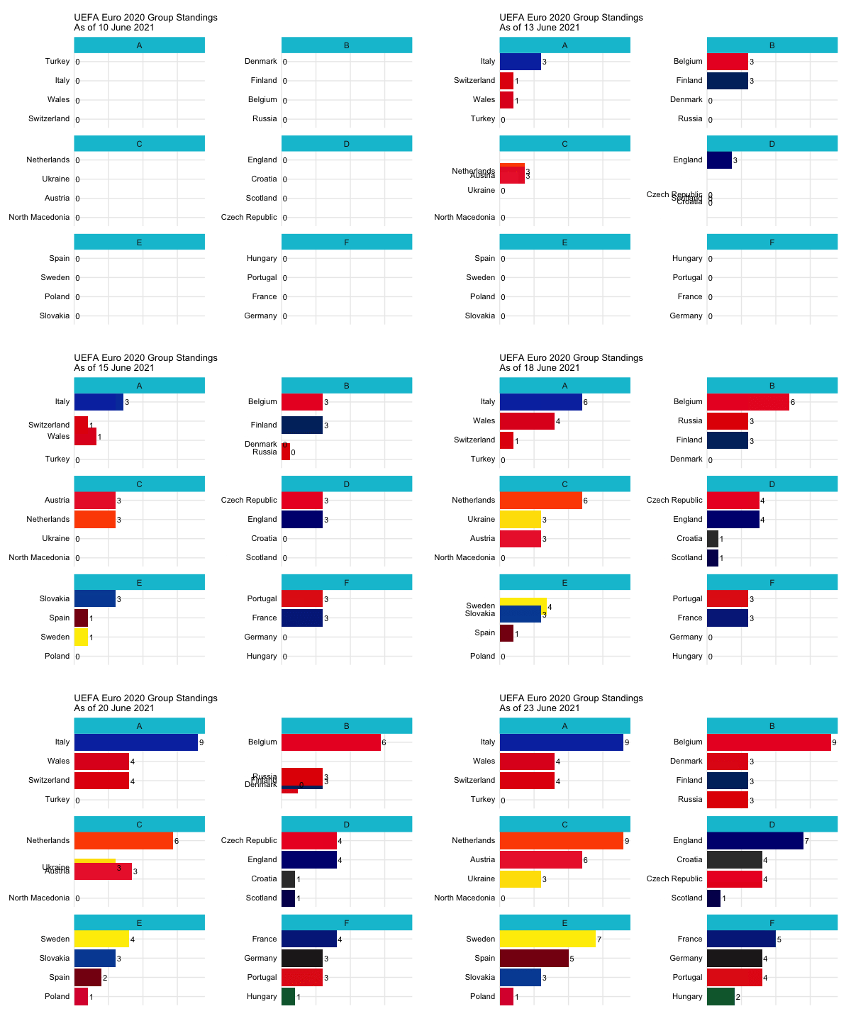
Lastly, the animation below shows how the group tables changed throughout the group stage of EURO 2020.
Show code
euro_groups <- read_csv("https://raw.githubusercontent.com/qntkhvn/funsies/main/animations/euro2020/euro_groups.csv")

colors <- c("#ED2939", "#eb192b", "gray22", "#ed1b2c",
            "#e32219","#00007e", "#002F6C", "#052789",
            "#231f20", "#0b663a", "#0A36AF", "#FF4F00",
            "#D20000", "#DC143C", "#e42518", "#e40303",
            "#05005b", "#034da3", "#880f14", "#ffec00",
            "#e4000f", "#E30A17", "#ffe000", "#e11a22")

a <- euro_groups %>%
  ggplot() +
  geom_col(aes(x = Rank, y = Points, group = Team, fill = Team),
           show.legend = FALSE) +
  geom_text(aes(x = Rank, y = 0, label = paste(Team, " ", sep = " "),
                group = Team),
            hjust = 1, size = 3, vjust = 0.35) +
  geom_text(aes(x = Rank, y = Points, label = as.character(Points)),
            hjust = -0.3, size = 3) +
  facet_wrap(~ Group, scales = "free", ncol = 2) +
  coord_flip(clip = "off", expand = FALSE) +
  scale_x_reverse() +
  ylim(c(0, 9.5)) +
  theme(
    axis.ticks.y = element_blank(),
    axis.ticks.x = element_blank(),
    axis.title = element_blank(),
    axis.text = element_blank(),
    plot.margin = margin(0.5, 0.5, 0.5, 2.7, "cm"),
    panel.spacing.x = unit(5.5, "lines"),
    panel.grid.minor = element_blank(),
    strip.background = element_rect(fill = "#00c1d5", color = "#00c1d5"),
    plot.title = element_text(size = 10)
  ) +
  scale_fill_manual(values = colors) +
  transition_states(Date, transition_length = 2, state_length = 1, wrap = FALSE) +
  ggtitle("UEFA Euro 2020 Group Standings\nAs of {closest_state}")

animate(a, nframes = 500, fps = 50, height = 480, width = 600, res = 95, end_pause = 200, duration = 12)
Tennis: Big Three
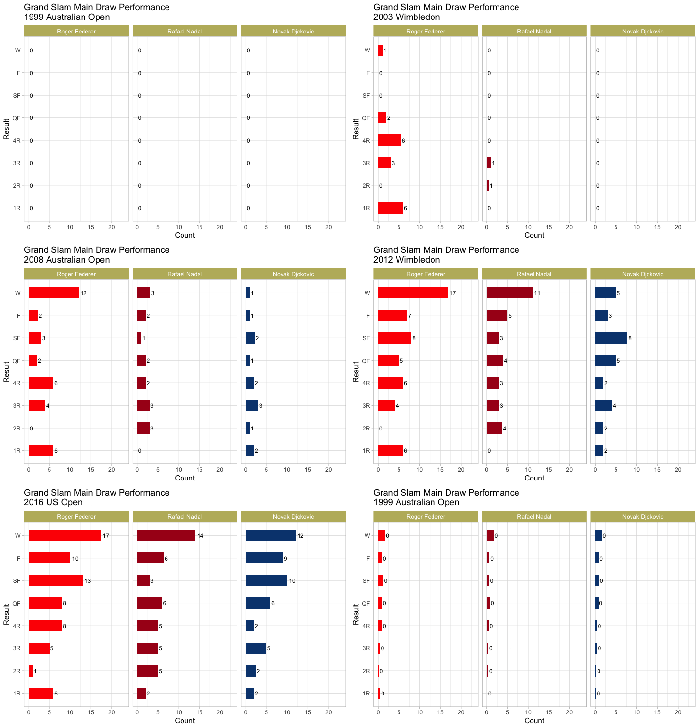
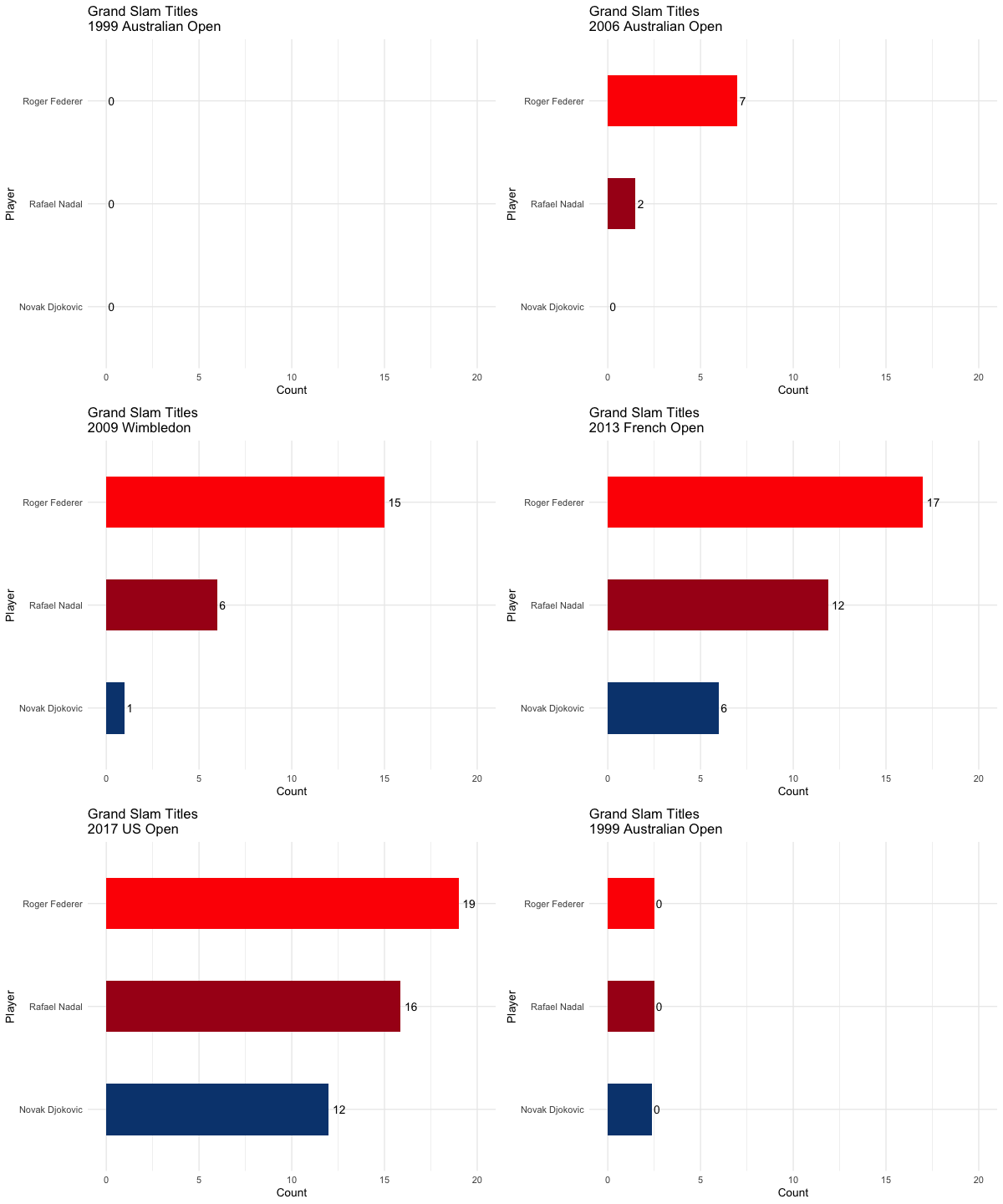
In addition to football, I also made a couple of tennis animations, both on Grand Slam performances of the famous Big Three - Federer, Nadal, and Djokovic. The two animated charts were made after the conclusion of the 2021 French Open, where Djokovic won his 19th Grand Slam title, and Novak is now only 1 trophy behind Roger and Rafa for the career grand slam winning record in the Open Era. I will be sure to update these plots after every Grand Slam tournament.
Grand Slam Titles
Show code
# for factor reordering
slams <- c(
  "1999 Australian Open",  "1999 French Open",  "1999 Wimbledon",  "1999 US Open",
  "2000 Australian Open",  "2000 French Open",  "2000 Wimbledon",  "2000 US Open",
  "2001 Australian Open",  "2001 French Open",  "2001 Wimbledon",  "2001 US Open",
  "2002 Australian Open",  "2002 French Open",  "2002 Wimbledon",  "2002 US Open",
  "2003 Australian Open",  "2003 French Open",  "2003 Wimbledon",  "2003 US Open",
  "2004 Australian Open",  "2004 French Open",  "2004 Wimbledon",  "2004 US Open",
  "2005 Australian Open",  "2005 French Open",  "2005 Wimbledon",  "2005 US Open",
  "2006 Australian Open",  "2006 French Open",  "2006 Wimbledon",  "2006 US Open",
  "2007 Australian Open",  "2007 French Open",  "2007 Wimbledon",  "2007 US Open",
  "2008 Australian Open",  "2008 French Open",  "2008 Wimbledon",  "2008 US Open",
  "2009 Australian Open",  "2009 French Open",  "2009 Wimbledon",  "2009 US Open",
  "2010 Australian Open",  "2010 French Open",  "2010 Wimbledon",  "2010 US Open",
  "2011 Australian Open",  "2011 French Open",  "2011 Wimbledon",  "2011 US Open",
  "2012 Australian Open",  "2012 French Open",  "2012 Wimbledon",  "2012 US Open",
  "2013 Australian Open",  "2013 French Open",  "2013 Wimbledon",  "2013 US Open",
  "2014 Australian Open",  "2014 French Open",  "2014 Wimbledon",  "2014 US Open",
  "2015 Australian Open",  "2015 French Open",  "2015 Wimbledon",  "2015 US Open",
  "2016 Australian Open",  "2016 French Open",  "2016 Wimbledon",  "2016 US Open",
  "2017 Australian Open",  "2017 French Open",  "2017 Wimbledon",  "2017 US Open",
  "2018 Australian Open",  "2018 French Open",  "2018 Wimbledon",  "2018 US Open",
  "2019 Australian Open",  "2019 French Open",  "2019 Wimbledon",  "2019 US Open",
  "2020 Australian Open",  "2020 French Open",  "2020 Wimbledon",  "2020 US Open",
  "2021 Australian Open",  "2021 French Open")

# scrape data from Wikipedia
player <- function(name) {
  wiki <- paste("https://en.wikipedia.org/wiki/", name, sep = "")
  html <- read_html(wiki)
  tables <- html_table(html)

  results <- tables[[4]] %>%
    filter(Tournament != "Win–Loss") %>%
    select(-SR, -contains("W")) %>%
    pivot_longer(!Tournament, names_to = "Year", values_to = "Result") %>%
    mutate(Result = ifelse(str_detect(Result, "\\[") == TRUE,
                           str_sub(Result, 1, nchar(Result) - 3), Result)) %>%
    filter(!(Result %in% c("", "NH", "Q1", "Q2", "A"))) %>%
    mutate(Result = factor(Result, levels = c("1R", "2R", "3R", "4R", "QF", "SF", "F", "W"))) %>%
    unite(Slam, c(Year, Tournament), sep = " ") %>%
    add_count(Slam, Result, name = "Count") %>%
    mutate(Slam = factor(Slam, levels = slams))

  results <- full_join(results, expand(results, Slam, Result)) %>%
    mutate(Count = ifelse(is.na(Count), 0, Count)) %>%
    arrange(Slam, Result) %>%
    group_by(Result) %>%
    mutate(Count = cumsum(Count),
           Player = name)
}

slam <- player("Roger_Federer") %>%
  full_join(player("Rafael_Nadal")) %>%
  full_join(player("Novak_Djokovic")) %>%
  mutate(Player = str_replace(Player, "_", " "),
         Player = factor(Player,
                         levels = c("Roger Federer", "Rafael Nadal", "Novak Djokovic")))

slam_anim <- slam %>%
  filter(Result == "W") %>%
  mutate(Player = fct_rev(Player)) %>%
  ggplot(aes(x = Count, y = Player, fill = Player)) +
  geom_col(width = 0.5, show.legend = FALSE) +
  scale_fill_manual(values = c("#08457e", "#aa151b", "red")) +
  geom_text(aes(label = as.character(Count)), hjust = -0.3) +
  ggtitle("Grand Slam Titles\n{closest_state}") +
  transition_states(Slam) +
  ease_aes("quadratic-in-out")

animate(slam_anim, nframes = 2160, fps = 50, height = 480, width = 600, res = 90, duration = 12)
Grand Slam Performances
Show code
slam_perf_anim <- slam %>%
  ggplot(aes(x = Count, y = Result, fill = Player)) +
  geom_col(width = 0.5, show.legend = FALSE) +
  geom_text(aes(label = as.character(Count)), size = 3, hjust = -0.3) +
  facet_wrap(~ Player) +
  xlim(c(0, 23)) +
  scale_fill_manual(values = c("red", "#aa151b", "#08457e")) +
  theme_light() +
  theme(strip.background = element_rect(fill = "darkkhaki")) +
  transition_states(Slam) +
  ggtitle("Grand Slam Main Draw Performance \n {closest_state}")

animate(slam_perf_anim, nframes = 2160, fps = 90, height = 500, width = 720, res = 100)
